VLOOKUP function – Microsoft Support

< img src =" https://support.content.office.net/en-us/media/4873755a-8b1e-497e-bc54-101d1e75d3e7.png" > Idea: Try utilizing the new XLOOKUP function, an improved variation of VLOOKUP that operates in any direction and returns exact matches by default

, making it much easier and easier to use than its predecessor. Use VLOOKUP when you need to find things in a table or a range by row. For example, search for a rate of a vehicle part by the part number, or discover a worker name based upon their staff member ID.

In its simplest form, the VLOOKUP function says:

= VLOOKUP( What you want to search for, where you wish to search for it, the column number in the variety including the worth to return, return an Approximate or Exact match– indicated as 1/TRUE, or 0/FALSE).

< img

• src =” https://support.content.office.net/en-us/media/4873755a-8b1e-497e-bc54-101d1e75d3e7.png” alt =” Your web browser does not support video. Install Microsoft Silverlight, Adobe Flash Player, or Web Explorer 9. “/ > Tips: The secret to VLOOKUP is to arrange your data so that the value you search for (Fruit) is to the left of

• the return value( Amount) you want to find. If you’re a Microsoft Copilot customer Copilot can make it even much easier to place and use VLookup or XLookup functions. See Copilot makes lookups in Excel simple.

Technical information

Use the VLOOKUP function to search for a worth in a table.

Syntax

VLOOKUP (lookup_value, table_array, col_index_num, [range_lookup]

For example:

• = VLOOKUP( A2, A10: C20,2, REAL)

• = VLOOKUP(” Fontana”, B2: E7,2, FALSE)

• = VLOOKUP( A2,’ Client Particulars’! A: F,3, FALSE)

How to get going

There are four pieces of information that you will need in order to build the VLOOKUP syntax:

1. The value you want to look up, likewise called the lookup worth.

2. The range where the lookup worth is located. Remember that the lookup value ought to always be in the first column in the variety for VLOOKUP to work correctly. For example, if your lookup worth is in cell C2 then your range need to begin with C.

3. The column number in the variety that contains the return value. For example, if you define B2: D11 as the range, you must count B as the very first column, C as the second, and so on.

4. Optionally, you can specify real if you desire an approximate match or FALSE if you want a precise match of the return value. If you do not specify anything, the default worth will always be TRUE or approximate match.

Now put all of the above together as follows:

= VLOOKUP( lookup value, variety containing the lookup worth, the column number in the range containing the return worth, Approximate match (TRUE) or Precise match (FALSE)).

Examples

Here are a couple of examples of VLOOKUP:

Example 1

< img src=" https://support.content.office.net/en-us/media/0d08ad32-9e64-4578-89af-4c85683394b6.png" alt="= VLOOKUP( B3, B2: E7,2, FALSE). VLOOKUP looks for Fontana in the very first column( column B) in the table_array B2: E7, and returns Olivier from the second column (column C) of the table_array. Incorrect returns a specific match."/ > Example 2

Example 3< img src =" https://support.content.office.net/en-us/media/28e39ac1-7552-4258-90d5-b38b37deb2b1.png" alt="= IF( VLOOKUP( 103, A1: E7,2, FALSE)=" Souse", "Located"," Not discovered "). IF checks to see if VLOOKUP returns Sousa as the last name of worker correspoinding to 103( lookup_value )in A1: E7( table_array ). Because the surname representing 103 is Leal, the IF condition is false, and Not Discovered is shown."/ > Example 4 < img src=" https://support.content.office.net/en-us/media/d9011e9d-e702-4fac-8434-1112907e96e3.png "alt ="= INT( YEARFRAC( DATE( 2014,6,30 ), VLOOKUP (105, A2: E7,5, FLASE),1)) VLOOKUP tries to find the birth date of the staff member corresponding to 109 (lookup_value )in the A2: E7 range( table_array ), and returns 03/04/1955. Then, YEARFRAC subtracts this birth date from 2014/6/30 and returns a worth, which is then transformed by INY to the integer 59. "/ > Example 5< img src =" https://support.content.office.net/en-us/media/dcfda044-79a4-40e1-a2c2-878a90ab8ecb.png" alt=" IF( ISNA( VLOOKUP( 105, A2: E7,2, FLASE) )= REAL, "Employee not found ", VLOOKUP( 105, A2: E7,2, FALSE)). IF checks to see if VLOOKUP returns a worth for surname from column B for 105 (lookup_value).

If VLOOKUP finds a last name, then IF will display the last name, otherwise IF returns Employee not found. ISNA makes certain that if VLOOKUP returns #N/ A, then the mistake is replaced by Employee not found, rather of #N/ A. In this example, the return worth is Burke, which is the surname corresponding to 105.”/ >

1. Integrate data from numerous tables onto one worksheet by using VLOOKUP You can use VLOOKUP to integrate multiple tables into one

2. , as long as among the tables has fields in common with all the others. This can be specifically beneficial if you need to share a workbook with people who have older versions of Excel that do

   

3. n’t support data features with multiple tables as information sources-

   • by combining the sources into one table and changing the information feature’s data source to the brand-new table, the information function can be utilized in older Excel variations( offered the data include itself is supported by the

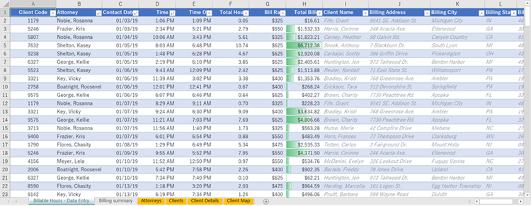
   • older variation).< img src =" https://support.content.office.net/en-us/media/e9b96547-1530-41fb-9eb2-c53c55aaa298.png" alt=" A worksheet with columns that use VLOOKUPto get data from other tables “/ > Here, columns A-F and H have worths or

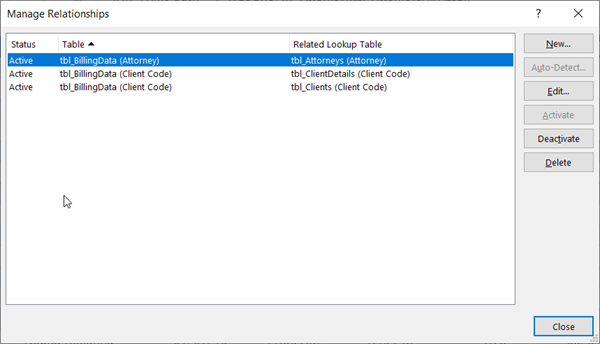
   • formulas that just use values on the worksheet, and the rest of the columns utilize VLOOKUP and the values of column A (Client Code) and column B( Attorney) to get data from other tables. Copy the table that has the common fields onto a brand-new worksheet, and give it a name. Click Data > Information Tools > Relationships to open the Manage Relationships dialog box.< img src=" https://support.content.office.net/en-us/media/0db6aff2-54bc-4051-8c2c-7be2c4d8f596.png" alt =" The Manage Relationships dialog box "/ > For each listed relationship, keep in mind the following: The field that connects the tables (listed in parentheses in the dialog box). This is the lookup_value for your VLOOKUP

4. formula. The Associated Lookup Table name. This is the table_array in your VLOOKUP formula. The field( column )in the Associated Lookup Table that has the data you want in

   your brand-new column. This info is disappointed in the Manage Relationships dialog- you’llneed to take a look at the Related Lookup Table to see which field you wantto recover. You want to note the column number( A= 1)- this is the col_index_num in your formula. To add a field to the new table , enter your VLOOKUP formula in the very first empty column utilizing the info you collected in step 3.

   In our example, column G uses Attorney (the lookup_value )to get the Expense Rate information from the 4th column (col_index_num= 4) from the Attorneys worksheet table, tblAttorneys( the table_array),

5. with the formula= VLOOKUP ([ @Attorney], tbl_Attorneys,4, FALSE). The formula might likewise utilize a cell reference and a variety reference. In our example, it would be= VLOOKUP (A2, ‘Attorneys’! A:D,4, FALSE). Continue including fields until you have all the fields that you require. If you are attempting to prepare a workbook containing information features that use several tables, alter the data source of the information include to the new table

. Typical Problems

Finest practices

Required more aid?

You can constantly ask an expert in the Excel Tech Community or get support in Neighborhoods.

See Likewise

XLOOKUP function

Video: When and how to use VLOOKUP

Quick Recommendation Card: VLOOKUP refresher

How to remedy a #N/ A mistake in the VLOOKUP function

Look up values with VLOOKUP, INDEX, or MATCH

HLOOKUP function

Find out how to utilize function VLOOKUP in Excel to find information in a table or variety by row. Our step-by-step guide makes vlookup in excel simple and efficient.