How to remedy a #N/ An error in the VLOOKUP function

< img src=" https://support.content.office.net/en-us/media/4c03d834-100f-4a35-8896-3942dfe127ce.png "> This subject describes the most common VLOOKUP reasons for an incorrect result on the function and

offers recommendations for using INDEX and MATCH rather. Problem: The lookup worth is not in the first column in the table_array

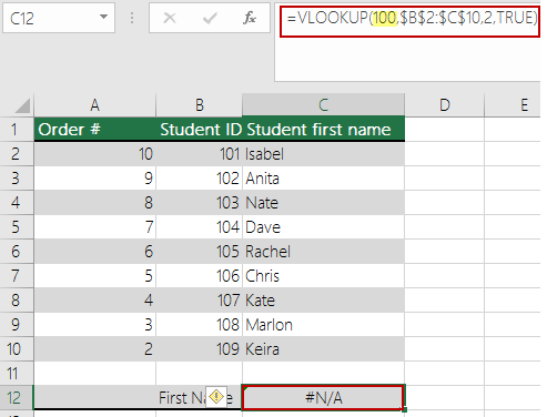
argument One restraint of VLOOKUP is that it can only look for worths on the left-most column in the table array. If your lookup worth is not in the very first column of the variety, you will see the #N/ A mistake.

In the following table, we wish to obtain the number of systems sold for Kale.

< img src= "https://support.content.office.net/en-us/media/4c03d834-100f-4a35-8896-3942dfe127ce.png" alt =" #NA mistake in VLOOKUP: Lookup worth is not in the first column of table selection “/ > The #N/ An error results since the lookup worth” Kale “appears in the 2nd column (Produce)

of the table_array argument A2: C10. In this case, Excel is searching for it in column A, not column B. Solution: You can try to fix this by changing your VLOOKUP to reference the correct column. If that’s not possible, then attempt moving your columns. That might also be extremely unwise, if you have large or complicated spreadsheets where cell worths are outcomes of other calculations– or possibly there are other logical reasons you merely can stagnate the columns around. The option is to utilize a mix of INDEX and MATCH functions, which can look up a worth in a column regardless of its location position in the lookup table. See the next section.

Think about utilizing INDEX/MATCH instead

INDEX and MATCH are good options for many cases in which VLOOKUP does not satisfy your requirements. The essential benefit of INDEX/MATCH is that you can search for a value in a column in any area in the lookup table. INDEX returns a value from a defined table/range– according to its position. MATCH returns the relative position of a worth in a table/range. Use INDEX and MATCH together in a formula to look up a worth in a table/array by specifying the relative position of the worth in the table/array.

There are several advantages of utilizing INDEX/MATCH instead of VLOOKUP:

• With INDEX and MATCH, the return value need not be in the exact same column as the lookup column. This is various from VLOOKUP, in which the return value has to remain in the specified range. How does this matter? With VLOOKUP, you need to know the column number that contains the return value. While this may not seem tough, it can be troublesome when you have a big table and need to count the variety of columns. Also, if you add/remove a column in your table, you have to recount and update the col_index_num argument. With INDEX and MATCH, no counting is required as the lookup column is different from the column that has the return value.

• With INDEX and MATCH, you can define either a row or a column in a variety– or specify both. This indicates you can look up worths both vertically and horizontally.

• INDEX and MATCH can be used to look up worths in any column. Unlike VLOOKUP– in which you can only look up to a worth in the very first column in a table– INDEX and MATCH will work if your lookup value is in the first column, the last, or throughout between.

• INDEX and MATCH use the versatility of making vibrant referral to the column which contains the return worth. This indicates that you can add columns to your table without breaking INDEX and MATCH. On the other hand, VLOOKUP breaks if you require to add a column to the table– given that it makes a static recommendation to the table.

• INDEX and MATCH uses more flexibility with matches. INDEX and MATCH can discover a specific match, or a value that is higher or lower than the lookup worth. VLOOKUP will just search for a closest match to a value (by default) or a precise value. VLOOKUP likewise presumes by default that the very first column in the table array is sorted alphabetically, and expect your table is not set up that way, VLOOKUP will return the first closest match in the table, which might not be the information you are trying to find.

Syntax

To build syntax for INDEX/MATCH, you need to utilize the array/reference argument from the INDEX function and nest the MATCH syntax inside of it. This take the type:

= INDEX( variety or recommendation, MATCH( lookup_value, lookup_array, [match_type]

Let’s use INDEX/MATCH to change VLOOKUP from the example above. The syntax will appear like this:

= INDEX( C2: C10, MATCH( B13, B2: B10,0))

In basic English it implies:

= INDEX( return a value from C2: C10, that will MATCH( Kale, which is someplace in the B2: B10 range, in which the return worth is the first worth corresponding to Kale))

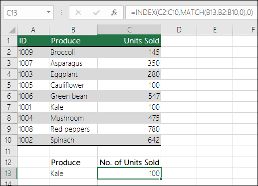
< img src=" https://support.content.office.net/en-us/media/40c79147-ea5b-419d-bd59-83b84f715a4f.png" alt=" INDEX and MATCH functions can be used as a replacement to VLOOKUP”/ > The formula searches for the first value in C2: C10 that corresponds to Kale( in B7 )and returns the worth in C7( 100), which is the very first value

that matches Kale. Issue: The precise match is not discovered When

the range_lookupargument is FALSE– and VLOOKUP is not able to discover a specific match in your data– it returns the #N/ A mistake.

Solution: If you are sure the appropriate data exists in your spreadsheet and VLOOKUP is not capturing it, take some time to validate that the referenced cells do not have actually hidden spaces or non-printing characters. Likewise, make sure that the cells follow the proper information type. For example, cells with numbers need to be formatted as Number, and not Text.

Likewise, consider using either the CLEAN or TRIM function to tidy up data in cells.

Problem: The lookup value is smaller than the smallest worth in the range

If the range_lookupargument is set to real– and the lookup value is smaller sized than the tiniest worth in the array– you will see the #N/ A mistake. Real try to find an approximate match in the array and returns the closest value lower than the lookup worth.

In the following example, the lookup value is 100, however there are no worths in the B2: C10 variety that are lower than 100; hence the error.

< img src="https://support.content.office.net/en-us/media/0d51a59f-d0c3-4f2d-ae90-ef6311624898.png" alt="N/An error

• in VLOOKUP when the lookup value is smaller sized than the tiniest worth in

• selection”/ > Solution: Fix the lookup value as essential. If you can not change the lookup worth and need greater versatility with matching worths, think about using INDEX/MATCH instead of VLOOKUP– see the area above in this article. With INDEX/MATCH, you can look up worths greater than, lower to, or equivalent to the lookup value. For more information on utilizing INDEX/MATCH rather of VLOOKUP, refer to the previous area in this topic.

Problem: The lookup column is not arranged in the rising order

If the range_lookup argument is set to TRUE– and one of your lookup columns is not sorted in the rising (A-Z) order– you will see the #N/ An error.

Service:

• Modification the VLOOKUP function to search for a precise match. To do that, set the range_lookupargument to FALSE. No sorting is needed for FALSE.

• Use the INDEX/MATCH function to search for a value in an unsorted table.

Problem: The value is a big drifting point number

If you have time values or big decimal numbers in cells, Excel returns the #N/ An error due to the fact that of floating point precision. Floating point numbers are numbers that follow after a decimal point. (Excel stores time values as drifting point numbers.) Excel can not keep numbers with huge floating points, so for the function to work properly, the drifting point numbers will require to be rounded to 5 decimal locations.

Solution: Reduce the numbers by rounding them up to five decimal locations with the ROUND function

Required more aid?

You can always ask a specialist in the Excel Tech Community or get support in Neighborhoods.

See Also

Correct the #N/ A errorin the VLOOKUP function.